The reliable mapping of species richness is a crucial step for the identification of areas of high conservation priority, alongside other value and threat considerations. This is commonly done by overlapping range maps of individual species, which requires dense availability of occurrence data or relies on assumptions about the presence of species in unsampled areas deemed suitable by environmental niche models. Here, we present a deep learning approach that directly estimates species richness, skipping the step of estimating individual species ranges. We train a neural network model based on species lists from inventory plots, which provide ground truth data for supervised machine learning. The model learns to predict species richness based on spatially associated variables, including climatic and geographic predictors, as well as counts of available species records from online databases. We assess the empirical utility of our approach by producing independently verifiable maps of alpha, beta, and gamma plant diversity at high spatial resolutions for Australia, a continent with highly heterogeneous diversity patterns. Our deep learning framework provides a powerful and flexible new approach for estimating biodiversity patterns, constituting a step forward toward automated biodiversity assessments.

Since the very beginning of biogeographic research, the estimation and extrapolation of species diversity has been of foremost interest (von Humboldt, 1817; Arrhenius, 1921). It is well established that species diversity is distributed unevenly across space, generally following a latitudinal gradient, with increasing diversity from the poles toward the equator (MacArthur, 1965). On a regional level, it has been found that there are substantial differences in species richness among habitats, such as between a forested area and an open grassland (MacArthur, 1965). These observed spatial patterns have led to the formulation of three levels of species diversity: alpha, beta, and gamma diversity (Whittaker, 1960).

Alpha diversity refers to diversity on a local scale, describing the species diversity (richness) within a functional community. For example, alpha diversity describes the observed species diversity within a defined plot or within a defined ecological unit, such as a pond, a field, or a patch of forest. The scale of such ecological units depends on the organism group of interest; while for birds a defined forest or grassland transect of several hundred m2 to several km2 may be appropriate to describe a species community, for insects this could be a single tree. For plants, alpha diversity is often equated to the count of species identified during the inventory of a vegetation plot of defined size (Revermann et al., 2016).

Beta diversity, on the other hand, describes the amount of differentiation between species communities. Unlike the other levels of species diversity, the exact interpretation and quantification of beta diversity varies substantially across studies (see Tuomisto, 2010a,b for a detailed review on this topic). Originally, beta diversity was defined as the ratio between gamma and alpha diversity (β=γ/α, sensu Whittaker, 1972). Today, one commonly used measure of beta diversity is the Sørensen dissimilarity index (see section “Materials and Methods” below for more detail), which captures spatial turnover as well as differences in diversity between sites (Koleff et al., 2003).

Gamma diversity describes the overall species diversity across communities within a larger geographic area. It is often summarized across biogeographic or political units, such as ecoregions or countries (Kier et al., 2005; Brummitt et al., 2021). Alternatively, studies commonly summarize gamma diversity within cells of a spatial grid of fixed cell-size (Goldie et al., 2010; Thornhill et al., 2016). While alpha diversity represents the actual species diversity that can be measured at a given site, gamma diversity more broadly and loosely describes the diversity of species that can be found in the whole area. Gamma diversity is the most communicated level of species diversity when referring to biodiversity hotspots, with tropical regions, in particular the Neotropics, showing the globally highest gamma diversity values (Raven et al., 2020). Alpha diversity, on the other hand, shows different areas of maximum diversity, dependent on the size of the area surveyed, with temperate grasslands showing among the highest species richness on small plots (Wilson et al., 2012).

While species diversity can be directly counted for small plot sizes, for example, during species inventories (alpha diversity), this requires much effort and thus cannot be scaled up to large areas or whole continents (gamma diversity). Therefore, many studies apply some form of modeling and estimation to derive diversity maps for larger areas. For example, gamma diversity is often inferred by modeling individual species distributions and adding these up to obtain the total number of species that occur in a given area (Mutke and Barthlott, 2005; Barthlott et al., 2007). However, this approach has been shown to introduce substantial errors, when cross-checking the diversity predictions with actual species counts in selected grid cells (Aranda and Lobo, 2011). A general shortcoming of these methods is that usually the data available is insufficient to reliably model the ranges for each individual species. This problem intensifies with the number of species in the target group for which to estimate diversity patterns. In some cases, total species diversity is extrapolated for larger groups, based on a selected subset of taxa with good data coverage, under the simplistic assumption that the diversity patterns revealed by these taxa are representative for others (Kier et al., 2005), which is however often not the case (Ritter et al., 2019).

Alternative approaches have been applied to the task of diversity estimation and mapping, which skip the step of modeling individual species ranges. These often involve using occurrence records, floras, and checklists to count the total number of species that has been recorded within large biogeographic regions (Mutke and Barthlott, 2005; Kreft and Jetz, 2007). While such approaches do not require modeling distributions of individual species, they are particularly vulnerable to biases in data collection, as some taxa may be better represented in some checklists and biodiversity repositories than others. This method assumes one single diversity value within each of the regions analyzed, without accounting for diversity differences within these (sometimes large) areas. Although it is possible to interpolate diversity values to a finer resolution using spatial autocorrelation of associated variables such as climatic predictors (Kreft and Jetz, 2007), such gap filling may be difficult to verify and often provides a false sense of confidence for data-poor regions.

With the emergence of continental and global vegetation plot databases (Chytrý et al., 2016; Bruelheide et al., 2019; Sabatini et al., 2021), a new data source with extended spatial coverage has become widely, providing point-estimates of species diversity within clearly delimited areas. Recently, Večeřa et al. (2019) showed the potential of machine learning methods (random forest models) to estimate the expected diversity for fixed size vegetation plots (alpha diversity), based on climatic and other predictors, when trained on alpha diversity data from vegetation plot databases. However, to our knowledge, available machine learning models cannot extrapolate vegetation plot data to larger areas and do not provide estimates of multiple metrics of biodiversity.

Here, we present a deep learning framework that uses neural network models to predict alpha, beta, and gamma diversity. The models are trained to predict plant diversity based on climatic and geographic predictors, measures of human impact, and sampling effort. Our approach requires neither specific distribution information about individual species, nor the manual extrapolation of species richness using methods such as species–area curves (Kier et al., 2005). Instead, our models inherently learn the species–area relationships, allowing prediction of the three diversity metrics at user-defined spatial scales. Our approach is purely data-driven and hypothesis-free, including the selection of the best neural network architecture, to avoid confirmation biases in terms of picking models whose diversity predictions best match previous expectations.

We selected plot-based vegetation survey data from Australia (vascular plants; Tracheophyta) to empirically test the effectiveness of our models in predicting diversity patterns and to validate our methodology. Australia, as an island continent, has the advantage of a clear delimitation of natural boundaries; it has high natural diversity and uneven biological sampling (González-Orozco et al., 2014; Cook et al., 2015; Laffan et al., 2016); high spatial heterogeneity with well-defined and contrasting biomes (Byrne et al., 2008, 2011; Macintyre and Mucina, 2021); a relatively well-documented vascular flora with reliable national databases (Sparrow et al., 2021)1 that feed into the Global Biodiversity Information Facility (GBIF)2; good climatic data3; and a large number of freely available plot-based vegetation records suitable for training deep learning frameworks (Sabatini et al., 2021).

The values of alpha, beta, and gamma diversity used in this study to train the neural network models were derived from vegetation plot data (species inventories). We downloaded these data from the sPlotOpen database (Sabatini et al., 2021), only using plots where all vascular plants had been assessed. This resulted in a total of 7,896 vegetation plots for Australia (Figure 1). For each vegetation plot, we compiled its area (which ranged from 50 to 10,000 m2) and the list of plant species identified in the plot (ranging from 1 to 115 species). From each of these sites, we compiled measures for alpha, beta, and gamma diversity as described in more detail below (Figure 1), which we used to train our models.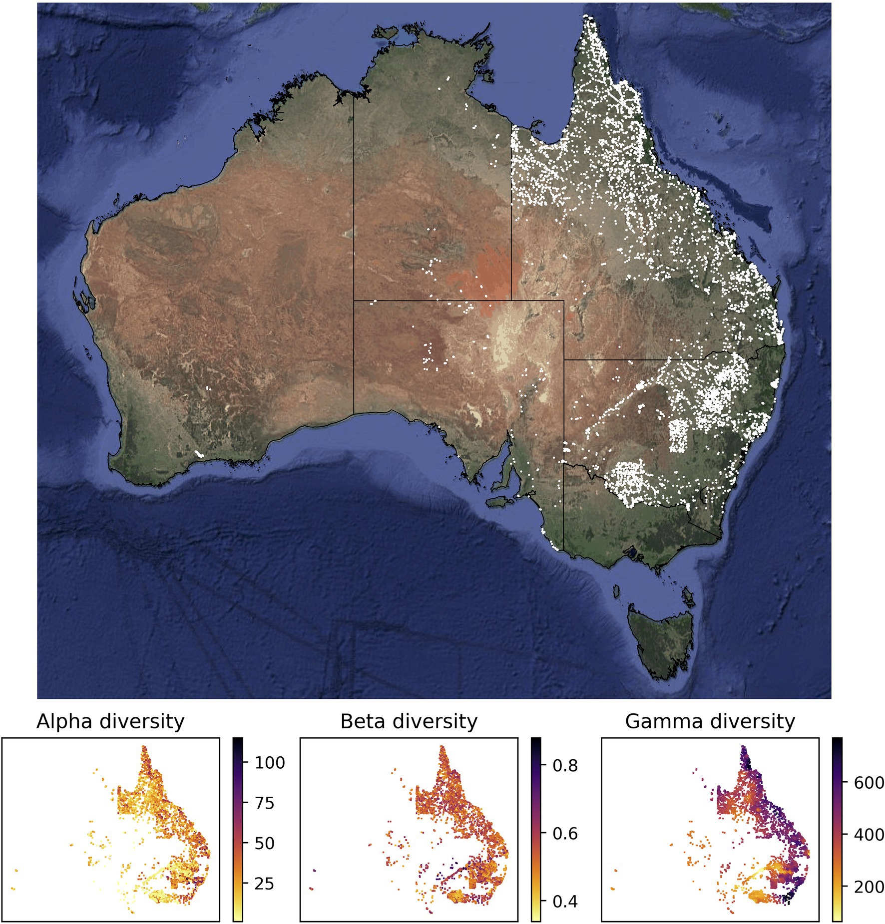

Figure 1. Sites with vegetation plot data used in this study for model training and evaluation. Most of the vegetation plot sites used in this study (white points, 7,896 sites) are located in the easternmost two Australian states Queensland (northeast) and New South Wales (center east). The panels below the map show the compiled measures of alpha, beta, and gamma diversity for all vegetation plot sites. The satellite image of Australia was downloaded via ggmap (Kahle and Wickham, 2013). The spatial scale of the alpha diversity estimates is defined by the plot size of the underlying vegetation plots and differs among sites. Similarly, the gamma diversity values are based on sets of 50 neighboring vegetation plots; depending on the spatial density of vegetation plots, these diversity values are therefore determined across different spatial scales. Both values, the size of the vegetation plot and the spatial scale of each gamma diversity estimate, are used as features in our models.

Calculating gamma diversity required the definition of a surrounding area, preferably containing other vegetation plots, to determine the overall diversity found within the cumulative species lists of several neighboring vegetation plots (Figure 2). To ensure that the same number of vegetation plots was used for calculating the gamma diversity of each site, we defined as the surrounding area a circle around each site encompassing exactly N nearest neighbors (vegetation plots). The gamma diversity for each site was then determined as the number of unique species names extracted from the species lists of the N nearest neighbors within the encompassing circle. After compiling diversity estimated for different values of N (Supplementary Figures S1–S7), we chose an N of 50 for all models in this study, as this value led to the best compromise between a visually discernible spatial structure in the resulting beta and gamma diversity values, while also highlighting regional heterogeneity (Supplementary Figure S3).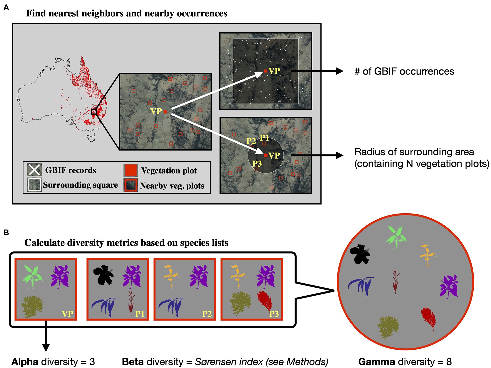

Figure 2. Calculation of diversity measures from vegetation plot data. For a given vegetation plot (VP, solid red square, panel A) we identified the N nearest neighboring vegetation plots in space (N = 3 in this example, represented by plots P1–P3). We exported the radius of the smallest circle encompassing all N neighbors as a feature for model training. Additionally, we exported the number of GBIF occurrences within a square of 10 × 10 km size around the given vegetation plot, as a measure of sampling effort in the general area. Having identified the nearest neighbors (P1–P3), we compared the species lists of these vegetation plots with the focal vegetation plot (VP, panel B). Alpha diversity represents the number of species found in the focal vegetation plot (VP), while gamma diversity represents the total diversity consisting of all species identified among the focal and neighboring vegetation plots. Beta diversity was calculated using the multiple-site Sørensen dissimilarity index (see section “Materials and Methods”), based on the differences in species composition found among the selected vegetation plots.

The radius of this encompassing circle varied between sites, depending on the proximity of other vegetation plots relative to the given site. The extent of the radius itself was used as a feature in our models, allowing the neural network to learn the expected associations between gamma diversity and the size of the area for which it was calculated (the species-area relationship), which we used later when making predictions with this model to adjust the spatial resolution of the predictions.

Finally, beta diversity was calculated using the multiple-site implementation of the Sørensen dissimilarity index (βsor), following the definition in (Baselga, 2010). For a given focal site j with N neighbors, we defined the focal site index as j = N + 1. We iterated through the N neighboring sites (i) and applied the formula:

with